Jupyter notebooks

Jupyter Notebook is an open-source web application for interactive computing. It allows the user to create and share digital notebooks that can contain code, visualizations, equations and text. It supports several different programming languages, including Python, Julia and many others.

I think Jupyter Notebooks are an excellent educational tool, as well as an ideal platform to share your research in a reproducible way. This is also mentioned in this article on the future of the scientific publishing. Here I show some of my projects related to Jupyter Notebooks.

Riemann Problems and Jupyter Solutions

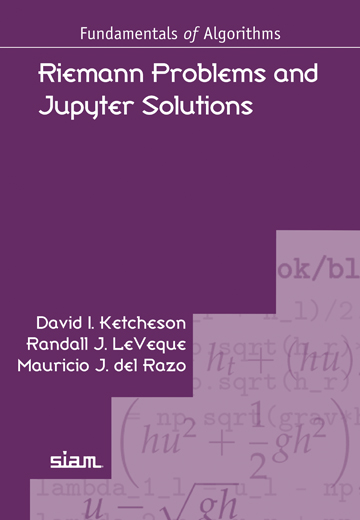
Together with David Ketcheson and Randall J. LeVeque, I co-authored an interactive book on Riemann problems. The book is completely constructed using Jupyter Notebooks to make use of animations, code and interactive applications as educational tools.

• D.I. Ketcheson, R. J. LeVeque, and M. J. del Razo. (2020) Riemann Problems and Jupyter Solutions. SIAM Fundamentals of Algorithms. [SIAM] [Binder] [html] [github]

To view the interactive book:

• Clone the GitHub repository and run the jupyter notebooks on your computer. The FA16 branch contains the notebooks corresponding to the printed book, while the master branch may have been updated.
• Run the notebooks on a server on binder (may take some minutes to launch)
• View the notebooks rendered as html (some interactive widgets do not work when viewed in html).

Book overview

Riemann problems consist of first-order hyperbolic partial differential equations (PDEs) with an initial condition given by two different constant values. Such PDEs arise when modeling wave propagation in applications such as fluid dynamics, acoustics, traffic flow, acoustics and elasticity. The solution of the Riemann problem captures essential information about such models, and it is the key ingredient in modern numerical methods for their solution. Below, we show an interactive example taken from the book; it consists of the simplest nonlinear conservation law, the Burgers’ equation $q_t+qq_x=0$, with a three-step initial condition. Its solution consists of two shocks, and it is obtained by solving two Riemann problems. Click the play button to see how the faster shock quickly catches up with the slowest one.

Once Loop Reflect

If the initial solution is changed, the behavior can change completely. In the example below, we changed to a different three-step initial condition. We can see how a rarefaction wave and a shock form. The rarefaction then interacts with the shock and modifies its propagation speed.

Once Loop Reflect

Below I show one more app developed for the book that illustrates the solution of the Riemann problem for the shallow water equations. Drag the left and right states in the first plot to change the initial condition of the Riemann problem, and drag the circle in the second plot to adjust the time.

For more details, check our full project on the GitHub repository..

Some interesting related links:

• In this link, you can watch Randy give a short talk on our project on PyData 2017.

• Here is a video on writing a book with Jupyter Notebooks from Jupytercon.

• Check out Jupyter Books, a tool that lets you build an online book using a collection of Jupyter Notebooks and Markdown files.

• Jake Vanderplas at the University of Washington has helped us out a lot with this project, and he also wrote this book using Jupyter Notebooks.

• PyEMMA is a Python library for the estimation, validation and analysis of Markov models derived from molecular dynamics data. A group of colleagues wrote a set of tutorials on Jupyter notebooks on how to use the software. See PyEMMA tutorials

• Here you can find a gallery of interesting Jupyter Notebooks.